Building a Neural Network from Scratch
Welcome!
In this post we will go through the proceedure of building a deep neural net from scratch using python and explore the underlying principles of neural networks in the process. The outline for this proceedure is as follows:
- Construct an example dataset from a sample distribution.
- Define the necessary components of the neural network and construct the corresponding functions.
- Assemble the functions into a neural network and train the model on the training portion of our example dataset.
- Use the model to predict features in the hold out portion of our example dataset.
1. Construct a Sample Dataset
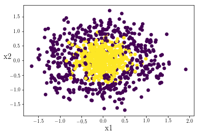
We will import the packages needed for this notebook and use the scikit-learn package to create a target shape data cluster.
import numpy as np
import matplotlib.pyplot as plt
from sklearn.datasets import make_circles
np.random.seed(10)
dataset = make_circles(1000,noise=.3,factor=.001)
X = dataset[0]
Y = dataset[1]
plt.scatter(X[:,0],X[:,1],c=Y)
plt.xlabel('x1',fontsize = 15)
plt.ylabel('x2', fontsize = 15, rotation = 0)
plt.show()

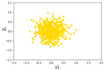
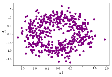
We can see explicitly that the data points in the center of the cluster are labeled 1, whereas those drawn from the encompassing fringe distribution are labled 0:
Y = np.reshape(Y,(1000,1))
sort_data = np.hstack((X,Y))
data_ones = sort_data[sort_data[:,2] == 1]
data_zeros = sort_data[sort_data[:,2] == 0]
plt.scatter(data_ones[:,0],data_ones[:,1],c='gold')
plt.xlabel('x1',fontsize = 15)
plt.ylabel('x2',fontsize = 15)
plt.xlim((-1.5,2))
plt.ylim((-1.5,1.5))
plt.show()

plt.scatter(data_zeros[:,0],data_zeros[:,1],c='purple')
plt.xlabel('x1',fontsize = 15)
plt.ylabel('x2', fontsize = 15, rotation = 0)

plt.show()

Traditional linear classifiers like LDA and logistic regression struggle with irregular data patterns such as these but simple neural networks are relatively good at these types of classifaction. Let’s get started building our network.
2. Define the Components of the Neural Network
In this section we will systematically lay out the components of a neural network and construct the accompanying functions necessary for our model.
If you are unfamiliar with neural networks here is a quick explanation:
The basic process of a neural network is to input a data matrix of features and observations, into a series of layers, each with multiple nodes. At each layer a new matrix is estimated using a weight matrix and a bias vector. The nodes at each layer determine the dimensions of these weight matrices and bias vectors.
This process of estimating new input matrices using the weight matrices and bias vectors is repeated until the final layer outputs a vector of predictions. This prediction vector is then compared to the vector of true labels. Recall that in our data the true label is either a
1or a0depending on which distribution the data was drawn from.
The network then slightly adjusts the weight matrices and bias vector in each layer, so that in subsequent iterations the network will output a prediction vector that more accurately predicts the true label vector. This process is repeated for many iterations until the prediction vector reaches a high enough accuracy to satisfy the researcher.
To start let’s consider our input data in matrix form:
\[\begin{align} \mathbf{X} = \mathbf{A}^{[0]} = \begin{bmatrix} \ a_{11}& \ldots& \ a_{1m} \\ \vdots& \ddots& \vdots \\ \ a_{n^{[0]}1}& \ldots& \ a_{n^{[0]}m} \end{bmatrix} \end{align}\]Each layer in our neural network requires an input matrix, $\mathbf{A}^{[l]}$. We can consider our data $\mathbf{X}$ as the first input, $\mathbf{A}^{[0]}$. Notice that $\mathbf{A}^{[0]}$ has dimensions $(n^{[0]},m)$. $n^{[0]}$ indicates the number of features in the dataset that we are using to make predictions, while $m$ is the number of oberservations or data points in our sample data. In subsequent layers, $n^{[l]}$ is the number of nodes in that layer.
At every layer $l$ we estimate a new matrix $\mathbf{Z}^{[l]}$ using the weight matrix and bias vector for that layer. The general layer matrix estimation is:
\[\begin{align} \underset{\small{(n^{[l]},m)}}{\mathbf{Z}}^{[l]} = \underset{\small{(n^{[l]},n^{[l-1]})}}{\mathbf{W}}^{[l]}\cdot \underset{\small{(n^{l-1},m)}}{\mathbf{A}}^{[l-1]} + \underset{\small{(n^{[l]},1)}}{\mathbf{b}}^{[l]} \end{align}\]where $n^{[l]}$ refers to the number of nodes at the $l$th layer, with the exception being $n^{[0]}$ which indicates the number of features in our dataset.
def forward_prop(A,W,b):
    '''
    Z = W*A + b
    '''
    Z = np.dot(W,A) + b

    return Z
Forward propagation through each layer requires us to input the estimation matrix $\mathbf{Z}$ into an activation function $g(z)$. The form of the activation function can vary between layers, and is one of several archetypes, such as a logistic or relu function. In this way the input matrix of the subsequent layer $\mathbf{A}^{[l]}$ is calculated:
\[\mathbf{A}^{[l]} = g(\mathbf{Z}^{[l]})\]The most commonly used types of activation functions are relu and logistic/sigmoid activation functions. Let’s define the relu activation function:
\[g(z) = \Bigg\{ \begin{matrix} \ z, & if \ z \geq{0} \\ \ 0, & if \ z < 0 \end{matrix}\]def relu(Z):
A = np.maximum(0,Z)
return A
And the logistic/sigmoid activation function:
\[\sigma(z) = \frac{1}{1\ + e^{-z}}\]def sigmoid(Z):
y = 1/(1 + np.exp(-Z))
return y
Let’s now define a function to input our data into and create the initial weight matrices and bias vectors for each layer:
def init_parameters(X, layer_list):
    '''
    This function takes in a dataset, X, with dimensions
    (n_0, m) where n_0 is the number of features of the
    dataset and m is the number of observations, and appends
    n_0 to a layer_list representing the number of nodes at
    each layer in the network. The length of the layer_list
    is the number of layers
    '''

    assert layer_list[len(layer_list)-1] == 1, 'last element of layer_list must be 1 (node)'

    parameters = {}


    n_0 = [X.shape[0]]  # number of features in dataset
    layer_list = n_0 + layer_list # add dimensions of features to layer_list


    L = len(layer_list)


    for i in range(1,L):
        parameters['W' + str(i)] = np.random.randn(layer_list[i],layer_list[i-1])
        parameters['b' + str(i)] = np.zeros([layer_list[i],1])

    return parameters
Quick Recap:
- The forward propagation algorithm operates by taking in an input matrix $\mathbf{A}^{[l-1]}$ and returning a new estimation matrix $\mathbf{Z}^{[l]}$.
- The estimation matrix is then passsed into an activation function $g(z)$ which yields the next input matrix, $\mathbf{A}^{[l]}$.
In a network with $L$ layers, the $L$th input matrix of the network is calculated as $\mathbf{A}^{[L]} = g(\mathbf{Z}^{[L]})$. In our data we are trying to predict a binary outcome: if the data point in question is from the inner or the outer distribution that we generated earlier. Therefore our output $\mathbf{Y}$ is a vector of ones and zeros with dimensions $(1,m)$. The matrix $\mathbf{A}^{[L]}$ has the same dimensions as our binary labels $\mathbf{Y}$ and contains our binary predictions for each of the observations (datapoints) in our data. The accuracy of these predictions is evaluated using a cost function. In this example we use a log-loss function. The log-loss is summed accross the $i \in {1,…,m}$ obervations:
\[\mathcal{L}(\mathbf{Y},\mathbf{A}^{[L]}) = -\frac{1}{m} \sum\limits_{i = 1}^{m} (y^{(i)}\log\left(a^{[L] (i)}\right) + (1-y^{(i)})\log\left(1- a^{[L (i)}\right))\]Vectorizing the cost function we have:
\[\mathcal{L}(\mathbf{Y},\mathbf{A}^{[L]}) = -\frac{1}{m} \left[ \ \begin{bmatrix} \ y^{(1)} \ \dots \ y^{(m)} \end{bmatrix} \begin{bmatrix} \ log(a^{[L](1)}) \\ \ \vdots \\ \ log(a^{[L](m)}) \end{bmatrix} - \begin{bmatrix} \ 1 - y^{(1)} \ \dots \ 1 - y^{(m)} \end{bmatrix} \begin{bmatrix} \ log(1 - a^{[L](1)}) \\ \ \vdots \\ \ log(1 - a^{[L](m)}) \end{bmatrix} \ \right]\]def log_loss(Y, A_L):
'''
Takes in Y vector (1, m) of labels and the
A_L vector (1, m) of predections for the Lth
layer and calculates the log loss function.
'''
m = Y.shape[1]
loss = (-1/m)*(np.dot(Y,np.log(A_L).T) + np.dot((1-Y),(np.log(1-A_L).T)))
loss = np.squeeze(loss)
return loss
In pseudo code, one iteration of the forward propagation algorithm is:
for $l$ in 1 to $L$:
calculate $Z^{[l]} = W^{[l]}A^{[l-1]} + b^{[l]}$
calculate $A^{[l]} = g(Z^{[l]})$
calculate cost function $\mathcal{L}(Y,A^{[L]})$
def forward_pass(parameters,X,Y):
    '''
    does a forward pass of the network and calculates
    the cost function
    '''
    Z_dict = {}
    A_dict = {}
    A_dict['A0'] = X

    L = len(parameters)//2

    for i in range(1,(L)):
        Z_dict['Z'+str(i)] = forward_prop(A_dict['A'+str(i-1)], parameters['W'+str(i)],
                                          parameters['b'+str(i)])
        A_dict['A'+str(i)] = relu(Z_dict['Z'+str(i)])

    Z_dict['Z'+str(L)] = forward_prop(A_dict['A'+str(L-1)], parameters['W'+str(L)], parameters['b'+str(L)])
    A_dict['A'+str(L)] = sigmoid(Z_dict['Z'+str(L)])

    cost = log_loss(Y, A_dict['A'+str(L)])

    return cost, Z_dict, A_dict
Great! We have our forward propogation algorithm constructed. Now we turn to back propagation. The back propagation algorithm is used to calculate how the cost function $\mathcal{L}$ changes with respect to each of the weight matrices $\mathbf{W}$ and bias vectors $\mathbf{b}$ in the layers of our network. We need to calculate those partial derivatives and use them to adjust the values in $\mathbf{W}$ and $\mathbf{b}$. This process is called gradient descent, and it is designed to minimize the cost function over many iterations, to increase the accuracy of our predictions $\mathbf{A}^{[L]}$ of the true labels in our data $\mathbf{Y}$.
We use chains of partial derivatives to obtain the partials of the cost function with respect to $\mathbf{W}^{[l]}$ and $\mathbf{b}^{[l]}$ for each layer $l$. Beginning with layer $L$ we have:
\[\begin{align} \frac{\partial\mathcal{L}}{\partial\mathbf{W}^{[L]}} & = \frac{\partial\mathcal{L}}{\partial\mathbf{A}^{[L]}} \cdot\frac{\partial\mathbf{A}^{[L]}}{\partial\mathbf{Z}^{[L]}} \cdot\frac{\partial\mathbf{Z}^{[L]}}{\partial\mathbf{W}^{[L]}} \implies \frac{\partial\mathcal{L}}{\partial\mathbf{W}^{[L]}} = \frac{\partial\mathcal{L}}{\partial\mathbf{Z}^{[L]}} \cdot\frac{\partial\mathbf{Z}^{[L]}}{\partial\mathbf{W}^{[L]}} \\ \\ \frac{\partial\mathcal{L}}{\partial\mathbf{b}^{[L]}} & = \frac{\partial\mathcal{L}}{\partial\mathbf{A}^{[L]}} \cdot\frac{\partial\mathbf{A}^{[L]}}{\partial\mathbf{Z}^{[L]}} \cdot\frac{\partial\mathbf{Z}^{[L]}}{\partial\mathbf{b}^{[L]}} \ \implies \frac{\partial\mathcal{L}}{\partial\mathbf{b}^{[L]}} = \frac{\partial\mathcal{L}}{\partial\mathbf{Z}^{[L]}} \cdot\frac{\partial\mathbf{Z}^{[L]}}{\partial\mathbf{b}^{[L]}}\\ \end{align}\]Note that $\frac{\partial\mathcal{L}}{\partial\mathbf{W}^{[L]}}$ and $\frac{\partial\mathcal{L}}{\partial\mathbf{b}^{[L]}}$ have the same dimensions as $\mathbf{W}^{[L]}$ and $\mathbf{b}^{[L]}$, respectively. To calculate the how the cost function changes with respect to $\mathbf{W}$ and $\mathbf{b}$ in subsequent layers, we recursively use the partials of the cost function from the previous layer:
\[\begin{align} \frac{\partial\mathcal{L}}{\partial\mathbf{W}^{[L-1]}} & = \frac{\partial\mathcal{L}}{\partial\mathbf{Z}^{[L]}} \cdot\frac{\partial\mathbf{Z}^{[L]}}{\partial\mathbf{A}^{[L-1]}} \cdot\frac{\partial\mathbf{A}^{[L-1]}}{\partial\mathbf{Z}^{[L-1]}} \cdot\frac{\partial\mathbf{Z}^{[L-1]}}{\partial\mathbf{W}^{[L-1]}} \implies \frac{\partial\mathcal{L}}{\partial\mathbf{W}^{[L-1]}} = \frac{\partial\mathcal{L}}{\partial\mathbf{Z}^{[L-1]}} \cdot\frac{\partial\mathbf{Z}^{[L-1]}}{\partial\mathbf{W}^{[L-1]}} \\ \\ \frac{\partial\mathcal{L}}{\partial\mathbf{b}^{[L-1]}} & = \frac{\partial\mathcal{L}}{\partial\mathbf{Z}^{[L]}} \cdot\frac{\partial\mathbf{Z}^{[L]}}{\partial\mathbf{A}^{[L-1]}} \cdot\frac{\partial\mathbf{A}^{[L-1]}}{\partial\mathbf{Z}^{[L-1]}} \cdot\frac{\partial\mathbf{Z}^{[L-1]}}{\partial\mathbf{b}^{[L-1]}} \ \implies \frac{\partial\mathcal{L}}{\partial\mathbf{b}^{[L-1]}} = \frac{\partial\mathcal{L}}{\partial\mathbf{Z}^{[L-1]}} \cdot\frac{\partial\mathbf{Z}^{[L-1]}}{\partial\mathbf{b}^{[L-1]}} \end{align}\]Thus, the recursively defined partials for any $\mathbf{W}^{[l]}$ and $\mathbf{b}^{[l]}$ are:
\[\frac{\partial\mathcal{L}}{\partial\mathbf{W}^{[l]}} = \frac{\partial\mathcal{L}}{\partial\mathbf{Z}^{[l]}} \cdot\frac{\partial\mathbf{Z}^{[l]}}{\partial\mathbf{W}^{[l]}} \\ \\ \frac{\partial\mathcal{L}}{\partial\mathbf{b}^{[l]}} = \frac{\partial\mathcal{L}}{\partial\mathbf{Z}^{[l]}} \cdot\frac{\partial\mathbf{Z}^{[l]}}{\partial\mathbf{b}^{[l]}}\]Calculating these partials can be pretty tricky; in a future post I will show how I derived the derrivative equations used in the backward propagation algorithm below:
def backward_pass(parameters,Y,Z_dict,A_dict):
    '''
    Takes the parameters W and b of each layer and
    calculates the gradient with respect to the cost
    function. Z and A matrices are input to calculate
    the partials and Y is is input to obtain a value
    for m, the number of sampes or observations in our
    dataset.
    '''

    dA_dict = {}
    dZ_dict = {}
    dParam_dict = {}

    L = len(parameters)//2
    m = len(Y)

    dA_dict['dA'+str(L)] = (1/m)*(A_dict['A'+str(L)]-Y)*(1/(A_dict['A'+str(L)]*(1-A_dict['A'+str(L)])))
    dZ_dict['dZ'+str(L)] = dA_dict['dA'+str(L)]*(A_dict['A'+str(L)]*(1-A_dict['A'+str(L)]))
    dParam_dict['dW'+str(L)] = np.dot(dZ_dict['dZ'+str(L)],A_dict['A'+str(L-1)].T)
    dParam_dict['db'+str(L)] = np.sum(dZ_dict['dZ'+str(L)],keepdims=True,axis=1)


    for i in range((L-1),0,-1):
        dA_dict['dA'+str(i)] = np.dot(parameters['W'+str(i+1)].T,dZ_dict['dZ'+str(i+1)])

        dZ_dict['dZ'+str(i)] = np.array(dA_dict['dA'+str(i)], copy = True)
        dZ_dict['dZ'+str(i)][Z_dict['Z'+str(i)] <= 0] = 0

        dParam_dict['dW'+str(i)] = np.dot(dZ_dict['dZ'+str(i)],A_dict['A'+str(i-1)].T)

        dParam_dict['db'+str(i)] = np.sum(dZ_dict['dZ'+str(i)],keepdims=True,axis=1)

    return dParam_dict
Quick Recap:
- For one loop of the forward propagation algorithm we can calculate how close our predictions $\mathbf{A}^{[L]}$ are to our actual labels in our data $\mathbf{Y}$.
- We want to tune our weight matrices $\mathbf{W}$ and bias vectors $\mathbf{b}$ so that our predictions $\mathbf{A}^{[L]}$ are closer to our labels $\mathbf{Y}$. Put another way, we are trying to minimize our cost function $\mathcal{L}$.
- To do this, we calculate how our cost function $\mathcal{L}$ changes with respect to each weight matrix $\mathbf{W}$ and bias vector $\mathbf{b}$ across our $L$ layers.
After calculating the partials with respect to the cost function $\mathcal{L}$ for all of our $\mathbf{W}$ and $\mathbf{b}$, we need to update the values within these weight matrices and bias vectors. Remember, we are trying to find values in each $\mathbf{W}$ and $\mathbf{b}$ to minimize the cost function $\mathcal{L}$. Therefore we are descending down the slope or gradient of the cost function. The learning rate is a value that determines how large of a gradient step each of the values in every $\mathbf{W}$ and $\mathbf{b}$ will take. When using a constant learning rate, the trade off is between time and accuracy. Smaller learning rates will cause the process of finding the minimum of the cost function to take computationally longer. This is because for each iteration of forward and backward propagation, the values within $\mathbf{W}$ and $\mathbf{b}$ are only changing by a very small amount. Put another way, we are making very small steps down the gradient of the cost function. However a relatively larger learning rate might cause us to take too large of a step and overshoot the minimum of the cost function, actually causing the cost function to increase. This can inadverdently cause the process of descending towards the minimum to take longer.
Let’s define a function to update the values in our $\mathbf{W}$ and $\mathbf{b}$:
def update_values(parameters, dParam_dict, learning_rate): ###
    '''
    takes in the parameters and updates
    '''

    L = len(parameters)//2

    for i in range(1,(L+1)):
        parameters['W'+str(i)] -= learning_rate * dParam_dict['dW'+str(i)]
        parameters['b'+str(i)] -= learning_rate * dParam_dict['db'+str(i)]

    return parameters
In pseudo code, one iteration of the backward propigation algorithm is:
for $l$ in $L$ to 1:
calculate $\frac{\partial\mathcal{L}}{\partial\mathbf{W}^{[l]}}$ and $\frac{\partial\mathcal{L}}{\partial\mathbf{b}^{[l]}}$
update $\mathbf{W}^{[l]} = \mathbf{W}^{[l]} - learningrate \cdot \frac{\partial\mathcal{L}}{\partial\mathbf{W}^{[l]}}$
update $\mathbf{b}^{[l]} = \mathbf{b}^{[l]} - learningrate \cdot \frac{\partial\mathcal{L}}{\partial\mathbf{b}^{[l]}}$
3. Assembling and Training the Network
We can now assemble the training function for our network. Our function will use the forward and backward propagation algorithms defined earlier to adjust the values in $\mathbf{W}$ and $\mathbf{b}$ to minimize the cost function $\mathcal{L}$.
def train_model(layer_list,X,Y,learning_rate,iterations):
    '''
    Builds a L layer binary classification neural network
    where L is the len(layer_list) and each value in
    layer_list specifies the number of nodes at that
    layer. Returns the parameters W and b which minimize
    the cost function within some error.
    '''

    parameters = init_parameters(X, layer_list)

    cost = 1 # set arbitrary cost =< 1

    for iteration in range(1,iterations):

        old_cost = cost

        cost, Z_dict, A_dict, = forward_pass(parameters,X,Y)

        dParam_dict = backward_pass(parameters,Y,Z_dict,A_dict)

        parameters = update_values(parameters, dParam_dict, learning_rate)

        if iteration in [1,2,3]:
            print('Iteration {}. Old cost is {}. Cost is {}.'.format(iteration,old_cost,cost))

        if(not iteration % 1000):
            print('Iteration {}. Old cost is {}. Cost is {}.'.format(iteration,old_cost,cost))

    return parameters
Let’s now choose a layer structure for our model and train it on our test data:
training_layers = [10,4,1]
Our training_layers variable indicates that our network will have 3 layers with 10 nodes in the first layer, 4 nodes in the second and a final single layer which will generate the prediction vector for each of our observations.
Recall from earlier that in our data $\mathbf{X}$ we have 1000 datapoints. Each of these is identified by two features, let’s call them x1 and x2. We now want to choose a portion of these datapoints to train our model on. We will arbitrarily choose the first 800 datapoints. This is refered to as our training_set. We also want to keep a portion of the datapoints in reserve. This prevents our model from becomming too attuned to predicting only the data that we presented it with, to the detriment of being able to predict other similiar but not identical sets of data. We will choose the remaining 200 datapoints as a holdout set. This is called our test_set. Let’s do that and check our dimensions:
training_set = X[0:800,].T
test_set = X[800:1001,].T

y_training_set = np.reshape(Y[0:800,], (800,1)).T
y_test_set = np.reshape(Y[800:1001,], (200,1)).T

print('The training_set has dimensions {}. \nThe test_set has dimensions {}.'.format(training_set.shape,test_set.shape))
print('The y_training_set has dimensions {}. \nThe y_test_set has dimensions {}.'.format(y_training_set.shape,y_test_set.shape))
The training_set has dimensions (2, 800).
The test_set has dimensions (2, 200).
The y_training_set has dimensions (1, 800).
The y_test_set has dimensions (1, 200).
Let’s now train our model using our training_layers and training_set:
np.random.seed(1)
predict_parameters = train_model(training_layers,training_set,y_training_set,learning_rate = 0.0005, iterations = 10001)
Iteration 1. Old cost is 1. Cost is 0.7915907142286972.
Iteration 2. Old cost is 0.7915907142286972. Cost is 0.7287529925292927.
Iteration 3. Old cost is 0.7287529925292927. Cost is 0.6985418397541265.
Iteration 1000. Old cost is 0.2314235697387047. Cost is 0.2314120460386395.
Iteration 2000. Old cost is 0.22881880114984401. Cost is 0.2288287806352107.
Iteration 3000. Old cost is 0.22662889790263158. Cost is 0.22663308811353614.
Iteration 4000. Old cost is 0.22398200275732244. Cost is 0.2239717800972103.
Iteration 5000. Old cost is 0.22239993494613244. Cost is 0.22232861167266244.
Iteration 6000. Old cost is 0.222114232153429. Cost is 0.22227546141609963.
Iteration 7000. Old cost is 0.22199988415862718. Cost is 0.22202476707642788.
Iteration 8000. Old cost is 0.22084172886809803. Cost is 0.2212719305418869.
Iteration 9000. Old cost is 0.22014454571887399. Cost is 0.22056276316549212.
Iteration 10000. Old cost is 0.21973503835360483. Cost is 0.2202900280690912.
We can see that even after Iteration 1000 the cost function has declined to 0.2314.... After this point the marginal decline in the cost function from each iteration is reduced. We should be cautious about continuing with more iterations after this point as our parameters $\mathbf{W}$ and $\mathbf{b}$ may be overfitted to our training set. Let’s also generate a set of parameters based on fewer iterations and then we will be able to compare which set of parameters better predict our test set. This will indicate if perhaps our first set of parameters based on 10000 iterations was somewhat overfit to our training data.
np.random.seed(1)
early_stop_predict_parameters = train_model(training_layers,training_set,y_training_set,learning_rate = 0.0005, iterations = 1001)
Iteration 1. Old cost is 1. Cost is 0.7915907142286972.
Iteration 2. Old cost is 0.7915907142286972. Cost is 0.7287529925292927.
Iteration 3. Old cost is 0.7287529925292927. Cost is 0.6985418397541265.
Iteration 1000. Old cost is 0.2314235697387047. Cost is 0.2314120460386395.
4. Predicting the Test Set
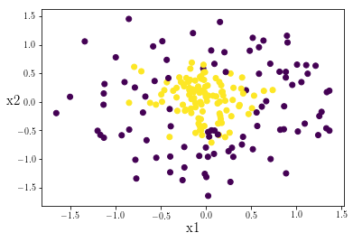
Let’s begin by checking out the datapoints in our test set. We want to ensure that it has a representative sample of inner points and outer points:
plt.scatter(test_set[0,],test_set[1,],c=y_test_set)
plt.xlabel('x1',fontsize = 15)
plt.ylabel('x2', fontsize = 15, rotation = 0)
plt.show()

The data looks balanced! Currently our prediction vector contains continous values. However we want to classify each of our points as either a 1 or a 0. Let’s quickly define a function to sort our continuous prediction values to either 1 or 0 based on if it is above or below 0.5:
def predict(predictions, labels):
    '''
    Takes in a set of continuous predictions and
    the actual lables of the data and returns a
    prediction accuracy
    '''
    assert(predictions.shape == labels.shape)

    predictions[predictions < .5] = 0
    predictions[predictions >= .5] = 1

    accuracy = np.sum(predictions == labels)/labels.shape[1]

    return accuracy
We can check if the early stop parameters yield a more accurate prediction on our test data:
reg_cost = forward_pass(predict_parameters,test_set,y_test_set)
print('The regular model has a cost value of {}'.format(np.reshape(reg_cost[0],(1,1))[0,0]),
      'and an accuracy ratio of {}.'.format(predict(reg_cost[2]['A3'],y_test_set)))
The regular model has a cost value of 0.2847705696329388 and an accuracy ratio of 0.875.
early_cost = forward_pass(early_stop_predict_parameters,test_set,y_test_set)
print('The early stop model has a cost value of {}'.format(np.reshape(early_cost[0],(1,1))[0,0]),
      'and an accuracy ratio of {}.'.format(predict(early_cost[2]['A3'],y_test_set)))
The early stop model has a cost value of 0.25496517602411756 and an accuracy ratio of 0.875.
We can see that our early stop parameters yielded a lower cost function value when applied to our holdout test data, but since we are classifying our continuous prediction outputs as either 0 or 1 it makes little difference as both sets of parameters yield the same model accuracy. Any further training iterations would likely overfit the model to the training data. Variables such as the number of layer and nodes, the learning_rate, and the number of iterations are referred to as hyperparameters. Our result suggests that for this dataset and these hyperparameters, the accuracy is essentially capped at 87.5%. However it’s certainly possible to tune hyperparameters to yield better predictive models. In a future post I will delve into how we can systematically optimize these hyperparameters.
5. Conclusion
Let’s recap what we learned:
- A deep neural network can be a good tool to predict labels in non-linear data.
- The network uses the forward and backward propagation algorithms to adjust the weight matrices and bias vectors at each layer of the network.
- As the weights and biases are tuned, the cost function approaches a minimum.
- If the model is trained on a given set of data for too many iterations, it can become very good at predicting the labels of the data it was trained on, to the detriment of predicting other samples of holdout or test data. This issue is called overfitting.
- An early stop of fewer iterations might yield a model with better predictive accuracy for other holdout or test data.
Thanks for reading!